Developing a brain inspired multilobar neural networks architecture for rapidly and accurately estimating concrete compressive strength

The human brain processes sensory information through a complex network of neurons, where different regions, known as lobes, manage specific aspects of incoming nerve impulses²⁶. This lobar processing allows the brain to handle complex tasks efficiently. Traditional ANNs, Fig. 1, typically rely on straightforward input-output pathways, which can be inadequate for handling large datasets and complex problems without significant computational overhead. These conventional ANNs often require deep networks to achieve satisfactory results, leading to lengthy training times and increased susceptibility to noise, which can compromise accuracy.

For a traditional ANN architecture, the process within a single layer $\:l$ can be mathematically represented as:

$$\:a^l=f\left(W^la^l-1+b^l\right)$$

(1)

where $\:a^l-1$ is the input (or activations from the previous layer); $\:W^l$ is the weight matrix; $\:b^l$ is the bias vector; $\:f$ is the activation function; $\:a^l$ is the output of layer $\:l$. For an ANN with $\:L$ layers, the final output $\:y$ is:

$$\:y=f^L\left(W^Lf^L-1\left(\cdots\:f\left(W^lx+b^l\right)\cdots\:\right)+b^L\right)$$

(2)

In order to address these limitations, ensemble learning neural networks (ELNNs) have been previously developed, as shown in Fig. 2. ELNNs aggregate multiple models through an ensemble layer to improve predictive performance. The ELNN’s operation involves multiple sub-models $\:i=\text1,2,\dots\:,M$, each producing an output $\:y_i$:

$$\:y_i=f_i\left(W_ix+b_i\right)$$

(3)

The final output of the ELNN is obtained by combining the outputs of all sub-models using an aggregation function $\:g$, such as a weighted sum:

$$\:y=\sum\:_i=1^M\alpha\:_iy_i$$

(4)

However, they can introduce interdependencies between models, potentially propagating noise and reducing training efficiency. Accordingly, this study develops an MLANN framework to replicate the brain’s biological mechanisms and functionalities for processing data structures in machine learning tasks.

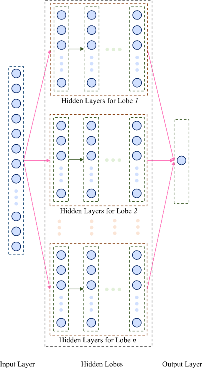
The proposed MLANN architecture, depicted in Fig. 3, is inspired by the brain’s lobar structure. In this regard, each lobe in the MLANN functions as an independent processing unit capable of addressing specific nonlinearities in diverse datasets. In the MLANN, the operation of each lobe $\:k=\text1,2,\dots\:,N$ can be described as:

$$\:z_k=f_k\left(W_kx+b_k\right)$$

(5)

where $\:z_k$ is the output of the $\:k$-th lobe; $\:W_k$ and $\:b_k$ are the weights and biases specific to that lobe; $\:f_k$ is the activation function used within the lobe.

The outputs of all lobes are then aggregated using a function $\:h$, such as the SoftPlus activation function:

$$\:y=log\left(1+e^\sum\:_k=1^Nz_k\right)$$

(6)

This design inherently promotes adaptability and scalability, enabling the incorporation of various types and functions within a single model without relying on deep layering. In the MLANN, each lobe consists of its own set of layers and neurons, allowing it to process input data independently before combining the outputs. This modular approach enhances flexibility and improves noise control during training compared to conventional methods. The independent lobes reduce the risk of noise propagation, as each lobe can specialize in learning different patterns or features within the data.

The MLANN algorithm, as described in Algorithm 1, outlines the procedure for training a model for regression tasks. While it follows many conventional ANN practices, it includes specific steps for this framework. Initially, the data is shuffled randomly to eliminate any inherent order that could bias the training process. The shuffled data is then divided into training and testing sets.

Both sets are normalized to ensure consistent scaling, which can improve the MLANN’s convergence speed and overall performance. The weights and biases of the MLANN are initialized randomly, with each lobe starting from a different seed. Each neuron in the MLANN employs an activation function to introduce nonlinearity into the model. During forward propagation, the input data passes through the MLANN, progressing through each lobe and layer, to produce a regression output. This process involves multiplying the inputs by the weights, adding biases, and applying activation functions at each neuron.

In the output layer, the SoftPlus activation function is utilized to aggregate the effects of all lobes, combining their outputs into a single regression result. Optimization techniques are then applied to minimize the loss function with respect to the network’s weights and biases^27,28. Finally, the optimized weights and biases are saved, and the model’s performance is evaluated using the testing dataset to assess its generalization capability.