Mechanical response characteristics and key technology of construction control of roof of long span string beam structure

Model construction

Element selection and boundary condition simulation

1. (1)

   Element s election

Upper Chord Members: the upper chord members of the beam-string structure are in the form of arched beams. To analyze bending moments and axial forces, these members are modeled as beam elements. Vertical Struts and V-Shaped Members: these components are modeled using truss elements. Lower Chord Cables: the lower chord cables are defined as tension-only elements, as they are designed to withstand only tensile forces.

1. (2)

   Boundary condition simulation

The beam-string structure has a unique configuration where the tensioning ends of the cables and the supports are not located at the same nodes. Based on the structural characteristics of the beam-string, the boundary conditions are simulated as follows. Support Conditions: One end of the structure is modeled as a fixed hinge support, while the other end is modeled as a sliding hinge support. Temporary Supports: at the locations of temporary supports, the nodal elastic support function is utilized. The temporary supports are converted into compression-only spring elements. Other Connections: all other parts of the structure are assumed to be rigidly connected.

Computational model

The three-dimensional numerical calculation model of the beam-string structure was established using the Midas Gen finite element software. The calculation model is shown in Fig. 3, The finite element model is based on Midas Gen 2024 (MIDAS Information Technology Co., Ltd.), where different colors represent different element types. The upper chord and diagonal braces of the beam-string structure are modeled using rectangular steel tubes, while the V-shaped struts and vertical struts are modeled using circular steel tubes. The lower chord cables are made of high-vanadium sealed strands. Considering that the overall structure undergoes large displacements with small strains during the tensioning process of the beam-string, a nonlinear analysis control method was adopted. The geometric nonlinearity type was selected, and the Newton–Raphson method was used for the calculation. The number of loading steps and the iteration count within each substep were set. To fully capture the nonlinear behavior of the structure, a relatively large number of substeps was used for each load step. The elastic modulus of the steel members in the beam-string structure is 2.06 × 10⁵ MPa, and the elastic modulus of the cables is 1.60 × 10⁵ MPa. The Poisson’s ratio for all components is 0.31. The parameters of the beam-string structure components are shown in Table 2.

BSS roof numerical calculation model.

Implementation of the calculation process

This study focuses on the computational analysis of the prestressing process of the cables in the beam-string structure, considering only the self-weight of the beam-string and the prestressing force of the cables. In Midas Gen, there are multiple methods to apply prestressing forces to the cables. In this study, the prestressing force is applied as follows: Load > Prestress Load > Initial Tension Load. This method of applying prestressing is suitable for simulating the staged tensioning process of the cables. It requires defining load cases for each stage of tensioning and then obtaining the combined results of cable forces and self-weight through load combinations.

The definition of the prestressing tension load combinations is shown in Table 3. These load combinations are used to define and calculate the load cases for the analysis. This approach ensures an accurate simulation of the staged tensioning process and provides a comprehensive understanding of the structural response under the combined effects of prestressing and self-weight.

The design value of the initial tension force for the cables is 1100 kN, and the application of the four-stage tensioning force can be divided into four phases. The static load cases include self-weight, PS1, PS2, PS3, and PS4. In the prestress load module, the initial tension forces are added sequentially as follows: PS1 initial tension force = 110 kN, PS2 initial tension force = 440 kN, PS3 initial tension force = 330 kN, and PS4 initial tension force = 275 kN. The finite element simulation of the construction process is mainly divided into the following steps: (1) Self-weight state of the beam-string structure on the support scaffolding; (2) First stage of prestressing application, first-stage cable tensioning, applying cable force to 110 kN; (3) Second-stage cable tensioning, applying cable force to 550 kN; (4) Third-stage cable tensioning, applying cable force to 880 kN; (5) Fourth-stage cable tensioning, applying cable force to 1155 kN (5% over-tensioning).

Computational loads

The main load conditions considered include:

1. 1.

   Self-weight of the structure (GL), with a nodal amplification factor of 1.1 applied.

2. 2.

   Roof dead load (DL), set at 1.0 kN/m².

3. 3.

   Roof live load (LL), set at 0.5 kN/m².

4. 4.

   Wind load (WX), determined by Eq. (1), following the specifications in the Load Code for the Design of Building Structures [GB50009-2012].

5. 5.

   Temperature load, with roof temperature controlled between 12 and 36 °C.

The unique characteristics of the BSS require careful consideration of temperature and wind loads. Wind suction forces, in particular, may affect the prestress in the cables, making the calculation of wind load conditions especially critical. The standard value for wind load perpendicular to the building surface is given by:

where ω₀—basic wind pressure, μ_s—wind load shape coefficient, μ_z—height variation coefficient of wind pressure, βz—wind vibration coefficient at height.

In this case:

• Wind vibration coefficient βz is taken as 1.99,

• Height variation coefficient μ_z is 1.00,

• Shape coefficient μ_s is − 0.8,

• Basic wind pressure ω₀ is 1.05 kN/m².

Thus, the calculated wind load ω_k is:

In numerical simulations, self-weight is automatically applied by the software, while roof dead and live loads are converted to nodal loads. Wind loads are applied as line loads on the model elements.

Tensioning overview

The tensioning process for the BSS roof utilizes a two-unit symmetrical staged cyclic tensioning method. The stages are as follows:

• Stage 1: Pre-tensioning with 10% of the target prestress (110 kN),

• Stage 2: Tensioning with 50% of the target prestress (550 kN),

• Stage 3: Tensioning with 80% of the target prestress (880 kN),

• Stage 4: Tensioning with 105% of the target prestress (1100 kN).

The tensioning steps are illustrated in Fig. 4. Based on the actual construction sequence, an initial analysis of the structural performance under self-weight is conducted with the BSS supported on the temporary frames. This is followed by simulating the deformation of the entire BSS roof as prestress is progressively applied to the cables. To ensure consistency between the simulation results and the actual construction process, an additional 5% over-tensioning is applied throughout the four tensioning stages.

Cable prestress grading symmetrical tension.

Initial state calculation results and analysis of the BSS roof

The vertical displacement results of the upper chords after each stage of the staged tensioning of the BSS roof are shown in Fig. 5. The results of the analysis were generated by Midas Gen 2024 (MIDAS Information Technology Co., Ltd.). Under self-weight conditions, both ends of each BSS unit exhibit downward deflection, with a maximum deflection of 18.6 mm, corresponding to a ratio of 18.6/646,000 = 1/34,000, which meets the deflection criterion of no more than 1/250 for steel structures. The deflection of BSS units located at the roof’s edges, namely BSS1 and BSS8, is relatively smaller.

Calculation results of tensile vertical displacement: (a) gravity; (b) Level 1 tensioning (10%); (c) Level 2 tensioning (50%); (d) Level 3 tensioning (80%); (e) Level 4 tensioning (105%).

After full pre-tensioning of the cables, the structure remains primarily influenced by self-weight, with minimal displacement changes across the BSS units. Following the second tensioning stage, noticeable displacement changes occur at both tensioned ends of the BSS units, with a maximum vertical displacement of 14.1 mm on the left tensioned end and 11.2 mm on the right, while the midspan region remains largely unchanged.

During the third tensioning stage, the BSS begins to develop an upward camber, with an increase in vertical displacement at the right tensioned end. After the fourth tensioning stage, each BSS unit achieves a cambered form, lifting off from the support frames. The maximum midspan displacement is located at the midspan of BSS3 and BSS6, with a peak value of 20.7 mm, which equates to a ratio of 20.7/646,000 = 1/30,761, satisfying the camber requirements as per structural standards.

Due to the significant changes observed at the midspan of the BSS units, the displacement trends at each midspan during the tensioning process were selected for comparative analysis. Figure 6a shows the midspan displacement variations of each BSS unit throughout the staged tensioning phases. The figure indicates that the overall midspan camber of each BSS unit is symmetrical, with the most noticeable displacement changes occurring during the fourth tensioning stage. This highlights the significant impact of prestress application in the later stages on BSS displacement, necessitating strict control of cable forces during this phase.

Vertical displacement change curve: (a) comparison of midspan vertical displacement of each BSS unit (b) time-history curve of midspan vertical displacement for the first four BSS units.

Upon completing the tensioning of the BSS roof, the deformations of all units are nearly identical. Notably, the camber values of BSS1 and BSS8 at the edges are 15 mm, which is 5 mm less than other units, indicating a more substantial coupling effect and constraint at the edges. The deformation of the mid span of each span of the string beam is more obvious, but the difference in arch height is not significant.

Mechanical response characteristics and key technology of construction control of roof of long span string beam structure placements of BSS2 to BSS7 are relatively uniform after staged tensioning, with a consistent camber height of approximately 20.7 mm. Overall, the differences in midspan heights among the BSS units are minimal, and the roof elevation remains uniformly aligned, meeting standard requirements.

To analyze the coupling effects between BSS units at each tensioning step, the vertical displacement time history curves for the first four BSS units were extracted, considering the symmetry of the roof structure. This analysis allows for an understanding of the overall tensioning process and its effects. As shown in Fig. 6b, the displacement trends for the first four BSS units are similar, initially showing steady increases, followed by a ramp-up in the later stages. Given the symmetrical nature of the overall tensioning model, it is reasonable to infer that similar displacement trends apply to other spans as well.

By comparing BSS1 and BSS3, it is observed that the coupling effect between the BSS units is weaker in the edge spans, while the tensioning influence is more pronounced in the central units. During in-situ tensioning, the BSS units exhibit mutual influence, with varying degrees of displacement impact on adjacent units as cable forces increase. The influence is most significant on adjacent BSS units, with closer units being more affected.

The horizontal displacement results for the BSS roof are shown in Fig. 7. It can be observed that, upon completing the tensioning process, the overall horizontal displacement of the structure is minimal. Horizontal displacement changes are primarily concentrated around the columns opposite the inclined braces, while displacement at the supports remains relatively minor.

Variation curve of support loading impact: (a) horizontal displacement variation of supports (b) support reaction force variation.

Under self-weight, due to the support frame, the load on the supports is light, resulting in an outward horizontal displacement of 5 mm. After tensioning, the displacement at the support changes to − 9 mm (inward), with the sliding support moving approximately 14 mm over the course of the process. Due to the effect of the inclined braces on the upper chord, the right inclined brace induces an outward horizontal displacement of 19 mm on the right concrete-encased steel column under self-weight. Following tensioning, this displacement reduces to 10 mm, while the left steel column exhibits an outward expansion of 11 mm. This indicates that while the tensioning process benefits the load-bearing capacity of the supports, it does exert some influence on the adjacent columns on both sides.

Figure 7a and b show the horizontal displacement and support reaction at the supports as functions of the tensioning stages, respectively. Both curves exhibit a similar trend, with values increasing from negative to positive. The horizontal displacement and support reaction values for each BSS unit are close at each tensioning stage, indicating that the coupling effect has minimal impact on the horizontal displacement and support reaction at the sliding supports during staged tensioning.

Initial state monitoring and analysis

Monitoring point arrangement

The initial state monitoring of the roof is used to verify the accuracy of the model analysis. Taking BSS1 to BSS4 as examples, each BSS unit has four monitoring points, located at the left tensioned end (Monitoring Point 1), midspan (Monitoring Point 2), right tensioned end (Monitoring Point 3), and sliding support end (Monitoring Point 4). These monitoring points are arranged identically across all spans, with a total of 32 monitoring points on the entire BSS roof.

Reducing the number of monitoring points helps minimize monitoring costs and accelerates the construction and monitoring process, while also simplifying data processing for key control points. Therefore, monitoring points in this project are primarily placed at the most critical locations. The layout plan of roof monitoring points was prepared using CAD 2021. The main monitoring point layout is shown in Fig. 8.

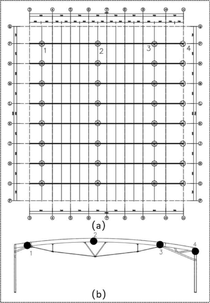
Monitoring point layout for BSS: (a) plan view of overall roof monitoring point layout (b) elevation view of monitoring point layout for a single BSS unit.

Displacement comparison analysis

To facilitate data processing and comparative analysis, monitoring data from a single BSS unit, specifically BSS1, is selected for comparison with its simulated data. The measured vertical displacement data at Monitoring Points 1, 2, and 3, as well as the horizontal displacement data at Monitoring Point 4, are extracted from BSS1. Time-history curves of the displacements at these four characteristic points across each prestress tensioning step are plotted, as shown in Fig. 9.

Comparison of simulated and monitored displacement time-history curves: (a) vertical displacement at left tensioned end (b) vertical displacement at right tensioned end (c) vertical displacement at midspan (d) horizontal displacement at support.

Since the horizontal displacement of the BSS structure is relatively unaffected by cable tensioning, the analysis primarily focuses on comparing the vertical displacement between monitored and simulated values at control points. Figure 9a and b reveal some differences between the two. Due to the asymmetry of a single BSS unit, the differing retraction distances at both tensioned ends, and the distinct support types on each side. There is a variation in vertical displacement between the left and right tensioned ends, although both generally show an upward trend.

Notably, Fig. 9b shows that the vertical displacement at the right tensioned end, which has a greater retraction distance, exhibits a marked increase during the early and mid-stages of tensioning, followed by a decrease in displacement in the later stages. Furthermore, Fig. 9c demonstrates that the monitored and simulated data at the midspan are closely aligned during the initial tensioning stages. In the third and fourth tensioning stages, the simulated values are slightly lower than the monitored values, but the tensioning deformation error remains within 10% across all stages. This trend aligns with the expected midspan deformation pattern, with the camber height at the midspan gradually increasing as the tensioning level progresses.

Additionally, Fig. 9d shows that the horizontal displacement of the right sliding support shifts from outward (positive) to inward (negative) as tensioning progresses, with a relatively small variation. This indicates that the inward retraction of the tensioned end has a beneficial effect on the load-bearing behavior of the support.

Calculation results and analysis of the BSS roof under load conditions

Due to the lightweight nature of the roof, the overall stiffness of the BSS structure is relatively low, making it susceptible to instability under unfavorable load distributions and extreme conditions. Therefore, stiffness and stability issues are critical in the analysis of this structure.

Under various load applications and combinations, the structure must satisfy the following control conditions:

1. 1.

   The strength and stability of structural components must meet code requirements;

2. 2.

   The maximum deflection must be less than L/200 (where L is the span of the BSS) to meet operational requirements and comply with the deformation requirements of the cladding system;

3. 3.

   No compressive stress should occur in the cables.

The calculation results for the three load conditions are shown in Fig. 10. Based on the vertical displacement contour maps under the three different load conditions, the following observations can be made:

1. 1.

   Condition 1 (Self-weight + Prestress + Dead Load + Live Load): The roof undergoes downward displacement, with vertical displacement concentrated in the central area. The middle four BSS units exhibit a displacement of up to 84 mm, while the displacement at the outermost roof sections is relatively smaller.

2. 2.

   Condition 2 (Wind Load): Under wind load, the vertical displacement of the structure decreases, with a maximum deflection of 37 mm, indicating an upward wind suction force acting on the roof structure.

3. 3.

   Condition 3 (Temperature Load of 36 °C): When subjected to a temperature load of 36 °C, the structure exhibits camber with a maximum height of 32 mm, demonstrating that the temperature load induces an upward camber force on the BSS.

Vertical displacement contour map (Unit: mm): (a) Condition 1 (b) Condition 2 (c) Condition 3.

These results highlight the need for careful consideration of stiffness and stability in the design and analysis of the BSS roof under various load conditions.

From Table 4, it can be concluded that the various data calculated under the three working conditions and load combinations show the following characteristics.

1. 1.

   Under Load Condition 1, due to the combined effects of dead and live loads, the roof undergoes an overall downward displacement, reaching 84 mm. The horizontal displacement at the supports and structural stress are higher than in other load conditions.

2. 2.

   Under Load Condition 2, the calculation results show that when wind load is applied, the suction force generated by the wind results in an upward force on the structure, reducing the vertical displacement of the roof. Additionally, it is observed that the cables remain engaged, indicating that the overall roof structure is in a safe state under this load condition.

3. 3.

   Under Load Condition 3, with the application of the maximum temperature load of 36 °C, the structure exhibits camber, with a camber value reaching 32 mm. Cable stress and compressive stress in the upper chords increase, but all values remain within safe limits, and the structural response complies with code requirements.

After completing the tensioning process, under the standard combination of dead load + live load, the maximum midspan deflection of the BSS is 84 mm, corresponding to a deflection-to-span ratio of 1/423. Under the wind suction load combination (dead load + wind suction load), the structure shows an upward vertical deformation of − 37 mm at the midspan, with a deflection-to-span ratio of 1/1025. Both conditions meet the design requirement of a deflection-to-span ratio not exceeding 1/250.

Stability analysis

Linear analysis

The stability analysis of the roof includes linear buckling analysis and nonlinear buckling analysis. When performing stability analysis of the BSS, a linear buckling analysis should be conducted first. The fundamental finite element equation for linear buckling analysis is as follows:

where \(K_{0}\) is the stiffness matrix of the structure, \(K_{\alpha }\) is the geometric stiffness matrix or the initial stress matrix of the structure, λ is the buckling eigenvalue, which represents the load proportionality factor (LPF), \(\Delta\) is the eigenvector, representing the displacement vector of each node in the buckling mode of the structure.

For the linear buckling analysis of this structure, prestress and self-weight are applied and kept constant. The dead and live loads are then proportionally increased. The first-order buckling mode of the structure is shown in Fig. 11, with an eigenvalue of 5.9. This indicates that, in an ideal linear buckling analysis, the large-span BSS roof can withstand approximately 5.9 times the combined dead and live load, giving a safety factor K of 5.9. This meets the requirement in Article 4.3.4 of the Technical Specification for Space Grid Structures, which mandates a K-value greater than 4.2.

1 first-order buckling mode.

Nonlinear analysis

However, linear buckling analysis assumes a defect-free structure with linear elastic material properties. In real engineering situations, factors such as construction errors and material imperfections typically result in an actual load-bearing capacity lower than that predicted by linear buckling analysis. To better approximate real conditions, a full-process nonlinear buckling analysis is necessary, accounting for both geometric and material nonlinearities. Nonlinear buckling analysis provides insight into the structure’s response from its initial state to ultimate load-bearing capacity and then through progressive loss of capacity, capturing changes in internal forces, displacements, and stresses.

In Midas Gen 2022, the arc-length method is used for nonlinear buckling analysis. During the nonlinear analysis, the geometric nonlinearity switch is enabled in the analysis step module, and the yield stress for Q355B steel is set to 355 MPa in the material properties. The load–displacement curve obtained from the nonlinear buckling analysis is shown in Fig. 12, with displacement contour plots for the structure under two load multiplication factors illustrated in Fig. 13.

Load–displacement curve.

Vertical displacement contour map under load combinations (Unit: mm): (a) 2.9 × load combination; (b) 3.2 × Load Combination.

The load reduction factor is a coefficient that appropriately discounts the design load in the structural design, taking into account the difference between the actual loading situation and the theoretical calculation model, as well as the reliability of the structure and other factors. From the load–displacement curve in Fig. 12, using the deflection generated in the initial state as the zero displacement reference, the vertical displacement of the midspan node increases with increasing load. When the load is less than 2.9 times the design load combination, the structure remains mostly in the linear elastic phase, and the load–displacement curve is approximately linear. When the load reaches 2.9 times the design load combination, the structure’s maximum deflection is 102.7 mm. As loading continues and reaches 3.2 times the design load combination, the maximum deflection is 149.6 mm. At this stage, a large area of the upper chord enters plasticity, the structure reaches its ultimate load-bearing capacity, can no longer carry additional load, and experiences instability and failure, with the load–displacement curve entering a descending phase.

Ultimately, the nonlinear buckling analysis shows that the structure can withstand approximately 3.2 times the combined dead and live load, yielding a safety factor KKK of 3.2, which meets the requirement of Article 4.3.4 of the Technical Specification for Space Grid Structures, mandating a KKK-value greater than 2.0.