
Optimization of roof slope, design and wood strength classes in timber Fink type truss

In this section, information regarding the study object will be addressed, namely, a timber truss roof structure, classified by ABNT NBR 868126 as a type 2 building, with accidental loads not exceeding 5 kN/m2.
Geometry
Due to its common geometry of symmetrical gable roofs, the Fink truss typology was adopted. The arrangement of the members depends on the roof slope and the type of roofing material used. In this study, the term ‘slope’ is used to describe the roof slope angle, expressed in degrees, which is equivalent to the term ‘slope’ as commonly used in structural geometry descriptions. Thus, technical catalogs of corrugated fiber cement sheets (commonly used in industrial/rural buildings) were consulted to establish basic guidelines for the design of these geometries27. The first guideline relates to the minimum slope, limited to 5° (9%). In practice, common slopes adopted for Fink-type trusses with corrugated fiber cement roofing systems range between 15° and 30°, based on manufacturer recommendations27. The expanded analysis from 5° to 41° in this study enables evaluation of both typical and boundary configurations, providing a broader understanding of material and structural behavior. It is also important to emphasize a minimum longitudinal overlap between sheets, specified by slope (α) ranges, as printed in Table 1.
Therefore, the geometries are designed by placing the sheets over the purlins, which are supported by the top chord, while respecting the longitudinal overlaps according to the slope. It is also permissible to have an overhang in the eave region, limited to values greater than 25 cm and less than 40 cm when gutters are not used.
The manufacturer’s catalogs also specify sheet lengths with their respective number of supports. In this study, only corrugated fiber cement sheets with a thickness of 6 mm and lengths of 122 cm, 153 cm, and 183 cm were used, with a minimum number of supports equal to 2.
In determining the position of the purlins located in the ridge region, a complementary ridge piece with a 300 mm flange and a minimum hole distance of 90 mm from its end was considered. For these considerations, the maximum D values given in Table 2 were respected.
In practice, common slopes adopted for Fink-type trusses with corrugated fiber cement roofing systems range between 15° and 30°, based on manufacturer recommendations. The expanded analysis from 5° to 41° in this study enables evaluation of both typical and boundary configurations, providing a broader understanding of material and structural behavior.Following the mentioned guidelines, the configuration of the members and group arrangement are depicted in Fig. 1.

Configuration of members and group arrangement.
To compare the trusses, the arrangement of the roofing sheets should be such that the number of members remains the same for any given slope. Therefore, starting from the minimum slope of 5° (9%), the maximum slope found was 41° (87%), which requires four sheets of 183 cm in length, a longitudinal overlap of 14 cm, and an approximate free overhang of 33 cm. Table 3 contains the values of longitudinal overlaps and arrangements of sheets used in the design of each geometry.
Loads
The actions and loadings acting on the structure were estimated with the aid of technical catalogs of fiber cement sheets and the ABNT NBR 612028 and ABNT NBR 612329 standards.
Dead loads
The dead loads acting on the truss are those arising from the self-weight of the timber structure and the roofing materials. The loading due to self-weight does not need to be inserted in a specific field since the algorithm automatically adapts minimum sections for each group of members, updating the self-weight of the structure at each iteration. The forces due to self-weight (Fj) are distributed to the load application points (joints “j” where the purlins are located). Their estimation is given by Eqs. (1) and (2), where ρap is the apparent density of the wood; Ai is the cross-sectional area of each member; ℓi is the linear length of each member; L is the truss span; dt is the distance between trusses; Ainf,j is the influence area of each joint receiving a purlin, and Fp is the concentrated self-weight of the purlin at the joint:
$${g}_{\text{dead-load}}=\frac{{\rho }_{\text{ap}}\cdot \sum_{i=1}^{n}{A}_{i}\cdot {{\ell}}_{i}}{L\cdot {d}_{t}}$$
(1)
$${F}_{j}=\left({g}_{\text{dead-load}}\cdot {A}_{{\text{inf}},j}\right)+{F}_{p}$$
(2)
Since the self-weight is automatically calculated, the only dead loads considered were those due to the weight of materials fixed to the structure, estimated at approximately 200 N/m2 with weight of 6 mm fiber cement sheets ≅ 180 N/m2 and sheet metal fittings ≅ 20 N/m2.
In the calculation of combinations of actions for the ultimate limit state (ULS), the dead loads were considered separately. For this situation, the load weighting coefficients (γ) printed in Table 4 were assumed, taken from item 6.1 of ABNT NBR 7190-125 and Table 1 of ABNT NBR 868126. It is worth mentioning that unfavorable effects occur when the dead loads act in the same direction as the main live load, while favorable effects occur in the opposite direction to the main live load.
Live load and wind load
The minimum live loads acting on roof structures are the accidental load and wind load. The accidental load corresponds to the minimum value of 250 N/m2 in horizontal projection, as recommended by item 6.4 of ABNT NBR 612028 for slopes equal to or greater than 3% (1.7°).
The wind action on the structure was quantified following the normative recommendations of ABNT NBR 612329, considering a rectangular building with a symmetrical gable roof. Figure 2 illustrates the floor plan, the cross-section, and the scheme of openings adopted for the building.

Floor plan and cross-section of building (dimensions in meters).
From Fig. 2, it can be observed that all dimensions of the building are fixed, except for the height of the roof (h), which varies according to the truss slope. Since the wind action on the building also varies with the height of the roof, to simplify the application of loads, it was decided to select the critical wind action among the 37 analyzed slopes. According to the ABNT NBR 612329, for a ratio between wall height and building width equal to or less than 0.5, the slope of 10° corresponds to the critical situation. Table 5 presents the parameters used in the calculation of the dynamic wind pressure for the slope of 10°, with a roof height equal to 0.882 m.
Therefore, the final dynamic pressures (q) are given by Eq. (3):
$$q = 0.613 \cdot v_{k}^{2} \Rightarrow \left\{ {\begin{array}{*{20}c} {0^\circ \,{\text{wind:}}\,\, 0.613 \cdot 33.25^{2} = 678 \,{\text{N}}/{\text{m}}^{2} } \\ {90^\circ \,{\text{wind:}}\,\, 0.613 \cdot 32.47^{2} = 646 \,{\text{N}}/{\text{m}}^{2} } \\ \end{array} } \right.$$
(3)
To quantify the wind action on the building, pressure was combined with the external and internal pressure coefficients. The external pressure coefficients (Ce) on the roof were determined using Table 7 of ABNT NBR 612329, considering the critical roof slope (10°) and the ratio between the wall height and the building width equal to 0.4. The values are illustrated in Fig. 3.

External shapes coefficients.
The internal pressure coefficients were quantified based on assumptions of dominant openings in different regions of the building (Fig. 2). For this purpose, fixed openings of 10 cm were considered on each face of the building, along with a 5 cm gap below the indicated gate in Fig. 2. Table 6 presents the internal pressure coefficients (cpi) for the critical assumptions prescribed in item 6.3.2 of ABNT NBR 612329. It should be emphasized that the objective was to extract the critical case of suction, which occurred at a wind angle of 90°, and the critical case of overpressure, which occurred at a wind angle of 0°.
Finally, the calculated value of the wind action on the building (wk) is shown in Eq. (4).
$$w_{k} = \left( {C_{e} – c_{pi} } \right) \cdot q \Rightarrow \left\{ {\begin{array}{*{20}l} {0^\circ \,{\text{wind:}}\,\, \left( { – 0.2 + 0.805} \right) \cdot 678 \cong 410\,{\text{N}}/{\text{m}}^{2} } \hfill \\ {90^\circ \,{\text{wind:}}\,\, \left( { – 1.2 – 0.690} \right) \cdot 646 \cong – 1220\,{\text{N}}/{\text{m}}^{2} } \hfill \\ \end{array} } \right.$$
(4)
In the ULS and serviceability limit states (SLS), the live load and wind load were considered separately, assuming the coefficients printed in Table 7, extracted from Tables 4 and 6 of ABNT NBR 868126.
Structural analysis and load combinations
Using the finite element method (FEM), the structural analysis model employed in the processing of the structure was that of a classical truss, i.e., perfectly hinged bar elements at their ends and subjected only to axial forces. Figure 4 illustrates the static scheme employed in all simulations.
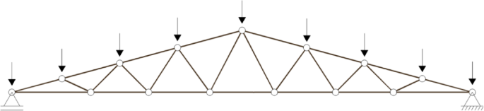
Static scheme of classic truss model.
The soliciting forces produced by each load described in section “Loads” need to be combined with each other to generate critical values for structural design. Using the weighting (γ) and reduction (ψ) coefficients, the design soliciting forces were obtained according to expressions from ABNT NBR 7190-125 for ULS under normal conditions, as transcribed in Eq. (5) below.
$${F}_{d}=\sum_{i=1}^{m}{\gamma }_{gi}\cdot {F}_{Gi,k}+{\gamma }_{q1}\cdot {F}_{Q1,k}+\sum_{j=2}^{n}{\gamma }_{qj}\cdot {\psi }_{0,j}\cdot {F}_{Qj,k}$$
(5)
Table 8 contains the three critical load combinations considered. The variable F in the second column of Table 8 corresponds to the characteristic design force due to the following factors: SW—self-weight; SH—roof sheets; AC—accidental loads; WD,o—wind overpressure; WD,s—wind suction.
It should be noted that the live actions (accidental and suction wind) are not grouped in Fd,3, as they are of opposite nature and have divergent directions, which does not lead to critical values of soliciting forces when summed in the same equation. Attention is also drawn to the 25% reduction in the forces resulting from wind action in Fd,3. The multiplication by 0.75 is in accordance with the recommendation of item 6.1 of ABNT NBR 7190-125, which considers the high strength of wood under short-duration loads when they represent the main variable action in isolation.
On the other hand, the combinations for SLS regarding structural deformations were calculated according to Eqs. (6) and (7), extracted from ABNT NBR 7190-125 corresponding to the long-duration class. In Eqs. (6) and (7), δinst represents instantaneous displacements, δfin represents final displacements, considering the effects of creep, and ϕ is the creep coefficient of wood, equal to 0.6 for sawn timber exposed to moisture class 1 (Uamb ≤ 65%).
$${\delta }_{\text{inst}}=\sum_{i=1}^{m}{\delta }_{{\text{inst}},Gi,k}+{\delta }_{{\text{inst}},Q1,k}+\sum_{j=2}^{n}{{\psi }_{1,j}\cdot \delta }_{{\text{inst}},Qj,k}$$
(6)
$${\delta }_{\text{fin}}=\sum_{i=1}^{m}{\delta }_{{\text{inst}},Gi,k}\cdot \left(1+\phi \right)+\sum_{j=1}^{n}{\delta }_{{\text{inst}},Qj,k}{\cdot \psi }_{2,j}\cdot \left(1+\phi \right)$$
(7)
Table 9 contains the four critical displacements combinations considered. The variable δinst in the second column of Table 9 corresponds to the instantaneous displacements to the following factors: SW—self-weight; SH—roof sheets; AC—accidental loads; WD,o—wind overpressure; WD,s—wind suction.
It is observed that the displacements resulting from wind action are disregarded in δfin because they are of short duration and do not affect the long-term normal use of the structure.
Design
Based on the calculated forces and displacements, the parameters for structural design followed the recommendations of ABNT NBR 7190-125, it is worth highlighting that the Brazilian standard was strongly inspired by Eurocode 530.
Strength classes, modification factors and purlin dimensions
For the components that will make up the roof purlins, the adopted wood species belongs to the Hardwoods group, class D40, defined in tests conducted on defect-free specimens. The characteristic values of compressive strength parallel to the grain (fc0,k), shear strength parallel to the grain (fv0,k), mean value of the modulus of elasticity in compression parallel to the grain (Ec0,m), and apparent density at 12% moisture content (ρap) were extracted from Table 2 of ABNT NBR 7190-125 and presented in Table 10.
Regarding the truss members, the processing of the four strength classes within the hardwoods group was chosen to obtain the optimal strength class along with the corresponding slope. Table 10 presents the values of strength, stiffness, and apparent density for each class within the hardwoods group.
According to the recommendations of ABNT NBR 7190-125, in the absence of characterization of tensile strength parallel to the grain (ft0,k) and bending strength (fb,k), it was assumed that ft0,k = fb,k = fc0,k.
The modification coefficients (kmod) were quantified based on the standard, varying according to the loading class, wood processing type, and moisture class. In this study, two live loads were estimated, with different loading classes: long-duration for accidental load and short-duration for wind load. To facilitate the estimation of the partial coefficient kmod,1 in all combinations, a long-duration loading was assumed, while the short-duration action (wind) was multiplied by 0.75 when it was the primary action in the combination, already included in Fd,3, Table 8. Therefore, assuming lumber exposed to an environment with relative humidity equal to or less than 65% (moisture class 1), the final modification coefficient (kmod) assumes a value of 0.70.
Prior to the truss design process, it is necessary to determine the sections that will compose the purlins. Although they are part of the self-weight of the wooden structure, they must be designed before the truss so that their actual loading is predicted and applied properly to the joints where they are located. These elements were treated as simply supported beams subjected to oblique bending, with a theoretical span equal to the distance between the trusses, limited to 3.0 m.
After the design process, it was found that a section of 60 × 120 mm meets all the verifications. Therefore, its self-weight is approximately 162 N (see Eq. (8)). Thus, at each joint where a purlin is located, a point load of 162 N was applied. It is worth noting that there are two purlins at the ridge joint, resulting in a value of 324 N at that location.
$${F}_{\text{purlin}}={\rho }_{ap}\cdot V=750\cdot \left(0.06\cdot 0.12\cdot 3.0\right)=16.2\,{\text{kg}}\cong 162\, {\text{N}}$$
(8)
Design standard for truss structures
The members that make up the truss structures are considered to have a full rectangular cross-section, as depicted in Fig. 5, where t, h, and L0 represent the thickness, height, and linear length, respectively.

Geometric representation and arbitrated variables for the member dimensions.
The cross-sectional area (Ai), slenderness ratio (λi), and radius of gyration (ri) of a generic member i are expressed by Eqs. (9), (10), and (11) respectively. Here, \({t}_{i}\) and \({h}_{i}\) correspond to the thickness and height of the member’s cross-section, respectively, and \({L}_{0,i}\) is the linear length of the member. \({I}_{i}\) represents the minimum moment of inertia about the critical axis, determined by selecting the dimension (thickness or height) that yields the smallest value. The thickness (\({t}_{i}\)) directly influences the radius of gyration (\({r}_{i}\)), thereby affecting the slenderness ratio (\({\lambda }_{i}\)). A lower slenderness ratio indicates a reduced risk of member buckling under axial compression, essential for ensuring compliance with the stability limits specified by ABNT NBR 7190-125.
$${A}_{i}={t}_{i}\cdot {h}_{i}$$
(9)
$${\lambda }_{i}={L}_{0,i}/{r}_{i}$$
(10)
$${r}_{i}=\sqrt{{I}_{i}/{A}_{i}}$$
(11)
Considering that the truss members are subjected only to axial forces, i.e., normal to the cross-section, it is of vital importance to verify their stability when subjected to compression, according to the criteria of ABNT NBR 7190-125. Using the slenderness ratio (λ), limited to values not exceeding 140, and the characteristic value of the modulus of elasticity measured in the direction parallel to the grain (calculated as 70% of Ec0,m), the relative slenderness ratio (λrel) in the critical direction is calculated, as per Eq. (12).
$${\lambda }_{\text{rel}}=\left(\lambda /\pi \right)\cdot \sqrt{{f}_{c0,k}/{E}_{\text{0,05}}}$$
(12)
The stability condition for axially compressed members is given by Eq. (13), where σNc,d is the design value of the normal compressive stress on the cross-section, and fc0,d is the design value of compressive strength parallel to the grain.
$$\frac{{\sigma }_{Nc,d}}{{k}_{c}{\cdot f}_{c0,d}}\le 1.0$$
(13)
The coefficients kc and k are obtained through Eqs. (14) and (15), respectively, where βc is the factor for structural members that meet the limits of alignment divergence, equal to 0.2 for lumber.
$${k}_{c}=\frac{1}{k+\sqrt{{k}^{2}-{{\lambda }_{\text{rel}}}^{2}}}$$
(14)
$$k=0.5\cdot \left[1+{\beta }_{c}\cdot \left({\lambda }_{\text{rel}}-0.3\right)+{{\lambda }_{\text{rel}}}^{2}\right]$$
(15)
In addition to stability verification, the safety condition for centrally compressed members is performed according to Eq. (16).
$${\sigma }_{Nc,d}/{f}_{c0,d}\le 1.0$$
(16)
In the design of axially tensioned members, the safety condition established by ABNT NBR 7190-125 is expressed by Eq. (17), where σNt,d is the design value of normal tensile stress on the cross-section, and ft0,d is the design value of tensile strength parallel to the grain.
$${\sigma }_{Nt,d}/{f}_{t0,d}\le 1.0$$
(17)
For the design of the truss and the application of design constraints, such as checking the ULS and SLS, it is necessary to obtain the design values of the mechanical properties of wood. As specified in ABNT NBR 7190-125, the design compressive strength parallel to the grain (fc0,d) and the effective value of the modulus of elasticity parallel to the grain (E0,ef) are determined by Eqs. (18) and (19) respectively.
$${f}_{c0,d}={k}_{\text{mod}}\cdot \left({f}_{c0,k}/{\gamma }_{w}\right)$$
(18)
$${E}_{0,{\text{ef}}}={k}_{\text{mod}}\cdot {E}_{c0,m}$$
(19)
where γw is the reduction coefficient for wood compressive strength, given a value of 1.4.
Furthermore, all structural failure modes were explicitly considered within the optimization process. The imposed design constraints ensured compliance with slenderness limits and buckling resistance criteria, addressing potential failure mechanisms such as compression buckling, lateral-torsional buckling, and global instability. The slenderness ratio was rigorously controlled according to ABNT NBR 7190-125, and the optimization algorithm systematically adjusted cross-sectional dimensions to mitigate instability risks. By integrating these considerations, the optimized truss designs achieve a balance between material efficiency and structural robustness, ensuring safe and reliable performance under varying design conditions.
It is worth noting that, in this study, both in-plane and out-of-plane buckling lengths were assumed to be equal to the linear length of each member (\({L}_{0}\)), as per a conservative 2D modeling approach without intermediate lateral bracing. While this simplification aligns with the design framework adopted by ABNT NBR 7190-125 and supports standardized member grouping, it may overestimate the risk of buckling in real-world scenarios. In practice, the incorporation of additional structural components—such as lateral bracing or a three-dimensional framework—could significantly reduce the effective buckling lengths, especially for longer compressed members near the ridge. Although such strategies were not considered in the current model, they represent a promising avenue for future research and practical refinement of timber truss designs.
Optimization algorithm
The algorithm used in this study was the Firefly Algorithm (FA), which was proposed by Yang31 and can be classified as a bioinspired probabilistic optimization method. This is a population-based method, meaning that more than one particle explores the search space in search of the optimal feasible solution. These methods use the concept of random variables for generating the initial population, which is a random event that respects the problem’s constraints31.
The theoretical inspiration for the design of this algorithm was drawn from the phenomenon of bioluminescence and the interactions among fireflies during mating. Therefore, the FA optimization method is based on the ability of fireflies to emit light and the ability of other individuals in the population to perceive this light.
When developing the algorithm, Yang31 defined some principles to assist in the development, including:
-
All fireflies have a single gender, and being of the same gender, they are attracted to each other.
-
The attraction ability of each firefly is proportional to its brightness, which decreases as the distance between individuals in the population increases.
With the generation of initial populations, the firefly (or design variable) starts a random walk, where \(\overrightarrow{x}\) moves according to an update function of design variables (\(\overrightarrow{\omega }\)), as described in Eq. (20), where \(\overrightarrow{x}\) is the vector of design variables; \(\overrightarrow{\omega }\) is the vector function for updating the design variable, and t is the number of iterations.
$${\overrightarrow{x}}^{t+1}={\overrightarrow{x}}^{t}+{\overrightarrow{\omega }}^{t}$$
(20)
From this new direction, new positions and potential candidate solutions are found to generate the optimal design point32. Thus, the movement between fireflies in the population at each step of the iterative process is given by Eq. (21).
$${\omega }^{t}=\beta \cdot \left({{\overrightarrow{x}}_{j}}^{t}-{{\overrightarrow{x}}_{i}}^{t}\right)+\alpha \cdot \left(\overrightarrow{\eta }-0.5\cdot \overrightarrow{\varepsilon }\right)$$
(21)
where β represents the attractiveness term between fireflies i and j; \({\overrightarrow{x}}_{i}\) represents firefly i; \({\overrightarrow{x}}_{j}\) represents firefly j; \(\overrightarrow{\eta }\) is the vector of random numbers between 0 and 1; α is the randomness factor, and \(\overrightarrow{\varepsilon }\) is a unit vector.
The randomness factor α follows an exponential decay behavior based on the number of iterations t, following the formulation proposed in Eq. (22), where θ is the decay constant with a value of 0.98.
$$\alpha ={\alpha }_{\text{min}}+\left({\alpha }_{\text{max}}-{\alpha }_{\text{min}}\right)\cdot {\theta }^{t}$$
(22)
As mentioned, the term β represents the attractiveness between fireflies in the swarm. This attractiveness is described according to Eq. (23), where β0 is the attractiveness for a distance r = 0; rij is the Euclidean distance between fireflies i and j, Eq. (24), and γ is the light absorption parameter (Eq. (25)).
$$\beta ={\beta }_{0}\cdot {\text{exp}}\left(-\gamma \cdot {{r}_{ij}}^{2}\right)\approx \frac{{\beta }_{0}}{1+\gamma \cdot {{r}_{ij}}^{2}}$$
(23)
$${r}_{ij}=\Vert {\overrightarrow{x}}_{i}-{\overrightarrow{x}}_{j}\Vert =\sqrt{\sum_{k=1}^{d}{\left({\overrightarrow{x}}_{i,k}-{\overrightarrow{x}}_{j,k}\right)}^{2}}$$
(24)
$$\gamma =\frac{1}{{\left({x}_{\text{max}}-{x}_{\text{min}}\right)}^{2}}$$
(25)
where k represents the k-th component of the design variable vector \(\overrightarrow{x}\); d is the number of design variables; xmax is the upper limit of the design variables, and xmin is the lower limit of the design variables.
The application of the FA or any other population-based probabilistic optimization method requires attention to the definition of algorithm parameters (attractiveness: β and γ; randomness: α).
The parameter γ characterizes the variation of attractiveness {γ ∈ [0, ∞)}, and its value is crucially important in determining the convergence speed and behavior of the algorithm. For most applications, this value ranges between 0.10 and 1031.
The pseudocode for the FA can be written following the structure presented in Fig. 6.

Pseudocode of Firefly Algorithm.
The Firefly Algorithm was selected for this study due to its proven effectiveness in handling constrained optimization problems with discrete variables, such as the selection of strength classes and sectional dimensions in timber trusses. Additionally, its search mechanism based on attractiveness and stochastic movement makes it suitable for global design space exploration under structural constraints. This choice is supported by Wang33, who conducted a comprehensive comparative study involving eleven popular metaheuristic algorithms, and demonstrated that the Firefly Algorithm achieves competitive results in terms of accuracy, stability, and convergence across diverse benchmark functions. While a direct comparison with alternative metaheuristics is not presented in this paper, we acknowledge that such analysis could complement this work and represent a valuable extension for future studies.
Handling constraints
In optimization problems applied to engineering, the use of constraints is necessary as they define the search space for the design variables34. The evaluation of constraints can be approached in two ways: indirect (or classical) and direct. In this study, the indirect or classical approach was adopted, which involves transforming a constrained optimization problem into an unconstrained optimization problem35.
In this research, the method of static exterior penalty was employed, which imposes penalty criteria. The criteria are based on evaluating the population with respect to the constraints, where a penalty function is applied to the solutions that violate the constraints. The exterior penalty coefficient Rp is used to activate this penalty. The complete pseudo-objective problem (penalized objective function) is expressed by Eq. (26).
$$W\left(\overrightarrow{x}\right)=FO\left(\overrightarrow{x}\right)+\sum_{j=1}^{m}{R}_{p}\cdot {{\text{max}}\left[0, {g}_{j}\left(\overrightarrow{x}\right)\right]}^{2}+\sum_{k=1}^{n}{R}_{p}\cdot {\left[{h}_{k}\left(\overrightarrow{x}\right)\right]}^{2}$$
(26)
In Eq. (26), (j, k) represents the j-th inequality constraint and k-th equality constraint, respectively; (m, n) are the total number of inequality and equality constraints, respectively; \(\overrightarrow{x}\) is the solution vector (random population); g and h are the set of inequality and equality constraints, respectively; and W(\(\overrightarrow{x}\)) is the penalized objective function.
Optimization algorithm parameters
Table 11 presents the input parameters of the FA based on the study by Pereira et al.24. In this research, a total population of 15 individuals will be considered, generated randomly. A total of 500 generations will be employed.
Objective function
The optimization problem aims to minimize the total weight of the structural system while considering constraints on joint displacements, mechanical strength of the members, and geometric criteria that may cause lateral instability in the structural system. The objective function of the system is expressed by Eq. (27), where Ai is the cross-sectional area of member i, ρi is the material density, L0,i is the length of member i in the truss, and n is the number of members in the truss.
$$FO\left({A}_{i},{\rho }_{i},{L}_{0,i}\right)=\sum_{i=1}^{n}{A}_{i}\cdot {\rho }_{i}\cdot {L}_{0,i}$$
(27)
As mentioned, the exterior penalty technique34,36 was employed to handle the constrained optimization problem. In this technique, the objective function is modified to become a pseudo-objective function, where gj represents the inequality constraints and hk represents the equality constraints. Equation (28) expresses the complete form of the adopted penalty method, while the penalized objective function W is presented in Eq. (29).
$$P\left(\overrightarrow{x}\right)=\sum_{j=1}^{m}{{\text{max}}\left[0, {g}_{j}\left(\overrightarrow{x}\right)\right]}^{2}+\sum_{k=1}^{n}{\left[{h}_{k}\left(\overrightarrow{x}\right)\right]}^{2}$$
(28)
$$W\left({A}_{i},{\rho }_{i},{L}_{0,i},{\overrightarrow{x}}_{i}\right)=FO\left({A}_{i},{\rho }_{i},{L}_{0,i}\right)+{R}_{p}\cdot P\left(\overrightarrow{x}\right)$$
(29)
where, it is worth noting that P(\(\overrightarrow{x}\)) represents the static exterior penalty function.
Type of variable adopted
In optimization problems, there are three types of variables that can be considered: continuous variables, discrete variables, and mixed variables (both continuous and discrete). Continuous variables can take infinite values within a given interval, while discrete variables have a finite set of allowed values (Fig. 7).

Graphic representation of continuous and discrete variables.
Due to the existence of predefined values for cross-sectional dimensions that are cataloged through current regulations and construction limitations, this research considered the nominal values for lumber found in ABNT NBR ISO 317937. Based on the nominal values specified in the mentioned standard, the following design variables are defined:
These values are presented in Table 12.
The truss members will be considered with simple sections of uniform thickness at all positions, varying only in height, and interconnected by means of metal plates. In the optimization process, truss members were grouped according to their structural roles, namely: bottom chord, top chord, and diagonals. While this approach streamlines modeling and enhances constructability, it does not compromise structural safety, as internal axial forces were evaluated using the envelope of all load combinations. Buckling checks were applied to all elements identified as compressed within this envelope, ensuring compliance with the stability and slenderness requirements specified by ABNT NBR 7190-125.
link


