Structural design, accuracy analysis, and mechanical calibration of a small two-component docking mechanism for large loads in space

Overall design of the docking system

The docking mechanism system consists of at least two single-component docking mechanisms. Each docking mechanism consists of an active side (AS) and a passive side (PS), which can automatically connect and disconnect. The extravehicular installation of a large space load is achieved by locking the active side (AS) to the passive side (PS). The active sides are securely mounted on the target load, while the passive sides are fixed to the extravehicular hull of the space station, as shown in Fig. 1. The design parameters based on the application requirements are provided in Table 1.

Dual-component docking mechanism.

In this design, the passive side is installed on the exterior of the space station module and is launched together with the module. During the upward launch, the exterior of the passive side is protected by the rocket fairing. Therefore, the passive side must fit within the limited space of Φ405 × 160 mm, formed by the space station module and the fairing, as shown in Fig. 2.

Schematic of the passive side uplink constraint environment.

The active side is mounted on the payload and launched alongside it. During docking, the robotic arm maneuvers the payload equipped with the active side. After the robotic arm positions the payload at the ideal docking location, it switches to zero-force mode, allowing the active side of the docking mechanism to capture the passive side. Since the robotic arm’s actual stopping position deviates from the planned position, the deviation range is ± 38 mm in all directions and ± 2° in each axis. Therefore, the capture range of the active side of the docking mechanism must accommodate this deviation.

The final positioning accuracy of the docking mechanism is ± 1.5 mm in each direction and ± 0.9° in each axis. During the docking process, the floating electrical connectors and floating fluid connectors must also be engaged simultaneously. The floating range of these connectors determines the required positioning accuracy of the docking mechanism.

This design aims to minimize the size of the active side while meeting the requirements for robotic arm deviations and large payloads. The target payload served by this docking mechanism has a mass of 4500 kg, and the available space for the active side on the payload is Φ465 × 450 mm.

Capture locking process: With the assistance of the space station’s extravehicular manipulator, the target load is moved into position. The vision camera on the active side and the vision target on the passive side help adjust the alignment, bringing the passive side of the docking mechanism into the capture range of the active side. The active side then drives the capture claw to secure the passive side, completing the coarse calibration. As the capture claw pulls the passive side closer, further fine calibration is performed using fine positioning pins and holes. This continues until the electrical and hydraulic circuits at both sides are docked and the arc rack is engaged. After the capture is completed, self-locking is achieved through a worm gear transmission mechanism, maintaining the locking state. The locking status is confirmed by the feedback from the micro-switch, indicating the locking state.

Unlocking and releasing process: The active side traction disc drives the claw to move in a straight line. When the gripping head of the claw contacts the separating surface of the passive side, it drives the passive side to separate from the active side axially. As the capture claw continues moving, it smoothly opens due to the interaction between its drive groove and the guiding shaft. The unlocking status is confirmed by the feedback from the micro-switch, indicating the unlocking state.

The positioning interface design incorporates a nested structure and utilizes a combination of V-groove positioning, pin hole guidance, and one-side two-pin positioning technology. The system sequentially meets the positioning requirements at each stage, achieving automatic centering and precise alignment, as illustrated in Fig. 3.

Positioning timing process.

Parametric design of the active side

The active side of each single component is shown in Fig. 4. It mainly consists of capture jaws, a power transmission mechanism, fine positioning pins, and a vision camera. The internal structure and sectional view of the active side are shown in Fig. 5. The process of capture and docking can be divided into several stages: capture, coarse calibration, fine calibration, and final locking. These stages are achieved through the interaction between the capture jaws on the active side and the passive side. The movement of the capture jaws is facilitated by the power transmission mechanism, which includes a motor, worm gear and worm, ball screw, and cam drive system. The motor serves as the motion and power output device, converting electrical energy into mechanical energy. The worm gear and worm not only reduce the motor speed but also increase the output torque, while also changing the direction of rotation by 90 degrees. The ball screw converts rotational motion into linear motion of the nut. The capture jaws are fixed on the nut platform, and the cam profile on the jaws enables their closing and vertical linear motion. The interaction between the capture jaws on the active side and the V-shaped groove on the passive side facilitates the initial capture and coarse alignment of the passive side. As the capture jaws pull the passive side closer, the fit between the two pins and holes further improves the docking accuracy. After fine calibration is completed, the alignment of the floating electrical and hydraulic connectors is achieved, followed by the final locking of the active and passive sides. Throughout this process, the coarse calibration and fine calibration stages proceed in sequence, with accuracy gradually increasing. In this design, the worm and worm gear allow for both forward transmission and reverse self-locking. The travel switch is used to limit the upper and lower limit positions of the traction disc, thereby controlling the degree of opening and closing of the capture jaws.

Internal schematic of the active end.

The active side geometric model is designed to meet installation envelope constraints, capture metrics, and other requirements. The geometric model of the active side is shown in Fig. 6. The parameters of the active side are defined in Table 2.

Geometric model of the active side.

The design of the active side model is related to the layout of the capture interface, the structural parameters of the active side, and the motion design of the claw. When the claw is fully opened, and the passive side moves randomly within the offset space, the capture claw does not touch the edges of the installation space. At the same time, the capture claw’s open state and the structural parameters of the active side must comply with the geometric model constraints. By analyzing the mechanical principles of the docking mechanism, a kinematic model of the mechanism was established for the fully extended state of the capture jaws, as shown in Fig. 6. Based on the docking mechanism’s design requirements (to accommodate robotic arm positioning deviations of ± 38 mm and ± 2°) and the kinematic relationships depicted in the figure, the axial tolerance Pm and radial tolerance dm were defined. These tolerances formed the basis for establishing the tolerance requirements and kinematic constraint equations of the mechanism, as presented in Eqs. (1) and (4). The four model parameters of the capture jaws (L1, L2, L3,and θ) are directly related to the tolerance space and the dimensions of the active side. The following constraint equations are derived for the design of the capture claw and the active side structure.

Parametric design of the passive side

The passive side of each single assembly is shown in Fig. 7, consisting primarily of a fine positioning hole, a V-groove, and a visual target. The V-groove is secured with a disc spring assembly near one end of the active side, while the other end has a detached surface. The primary function of the passive side’s V-groove is to provide a capture interface and guiding function for the capture jaws of the active side. Its geometric shape effectively limits unnecessary degrees of freedom, significantly improving the positioning accuracy and operational tolerance during the docking process. As the capture process progresses, the V-groove on the passive side and the capture jaws on the active side form a coarse alignment structure, allowing pose adjustments between the active and passive sides to achieve coaxial alignment, ensuring that the passive side remains within the capture area of the active side. The disc spring assembly, characterized by high stiffness, enhances the adaptability of the mechanism to space environments. When the capture jaws on the active side compress the load and the passive side, the disc spring assembly increases the system’s tolerance to environmental changes. When environmental conditions vary, such as temperature fluctuations or external disturbances, the pre-loaded disc spring assembly’s compression can elastically adjust, ensuring the load is consistently pressed against the passive side. After docking between the passive side and the active side, the disc spring applies an elastic thrust to the gripping head of the capture jaws, pushing it towards the active side. This ensures the worm gear and worm wheel are fully engaged, achieving self-locking through its structure. This enhances adaptability to space environments, including temperature fluctuations and micro-vibration conditions. Two sets of locating pins and holes are designed on the mating surfaces of the active and passive sides to achieve fine alignment. One of the holes is a long, bar-shaped slot to prevent over-positioning issues.

The passive side geometric model must meet constraints such as the upward mounting envelope with the cabin and the capture tolerance index. The geometric model of the passive side is shown in Fig. 8. The parameters of the passive side are defined in Table 3.

Geometric model of the passive side.

The passive end design is mainly determined by the V-groove opening height, width, active end geometry model and capture jaw structure. Based on the passive end geometry model, it is obtained that,

where HB is the height of the passive side.

Optimization of capture jaw parameters based on genetic algorithm

The genetic algorithm, a global optimization method based on natural selection and genetic variation, is utilized for multi-objective optimization^29,30. The impact of each design parameter on the optimization objectives is assessed through normalized sensitivity analysis. The optimization involves four design variables: L1, L2, L3, and θ. The optimization problem is treated as a single-objective optimization, where the objective function is the sum of the radial capture area (dm) and the axial capture area (Pm). Equal weights are applied to both terms to reflect their equal significance in the overall system performance.

The variables dm and Pm are defined in Eq. (1), with constants XA = 160 mm, HB = 60 mm, and hd = 64 mm. The mechanism must adhere to geometric constraints, including a minimum tolerance P of 38 mm in both axial and radial directions, a tolerance angle of 2°, and a maximum axial deviation of ∆Z = 17 mm post-overturning. The radial tolerance diminishes further:

Design variables are bounded with lower bounds (l_b) of [40, 200, 35, 60] and upper bounds (u_b) of [60, 280, 50, 80]. The initial guess for the variables is x₀=[40, 205, 40, 75]. The genetic algorithm used in this study is implemented using MATLAB’s ga function from the Optimization Toolbox. Key settings include a population size of 200 and a maximum of 500 generations. The algorithm uses real-coded chromosomes and a stochastic selection process to ensure global search optimization. After iterative optimization, the optimal solution is detailed in Table 4, where dm = 435.9999 mm and Pm = 124.501 mm. The optimized design is illustrated in Fig. 9.

Comparison chart of results before and after optimization.

The optimization results in a 4.01% improvement in the radial capture area and a 45.34% increase in the axial capture area. The sensitivity analysis is conducted to assess the impact of each design variable on the optimization objectives. This helps evaluate the robustness of the solution and highlight the most critical parameters, enabling a more targeted approach when reviewing the solution. This analysis sets the upper and lower bounds of each parameter as the range for evaluation, and calculates the effects on the optimization targets individually, as depicted in Fig. 10. Through the kinematic geometric model and sensitivity analysis results, it can be concluded that the design variables exhibit a linear relationship with the radial and axial capture areas.

Sensitivity analysis of each parameter.

A normalized sensitivity analysis is conducted by evaluating the impact of minor adjustments in each parameter on the objective. Incremental changes are applied separately to each parameter to compute the rate of change in the objective (f). Sensitivity is determined by normalizing these changes relative to the parameters’ adjustments and the optimized baseline value, then assessing each parameter’s relative influence on the outcomes^31,32,33. The findings are presented in Table 5.

To enhance the radial tolerance dm, increasing l₁ and l₂ is essential. Conversely, boosting the axial tolerance Pm primarily depends on l₃ and θ, though this may reduce dm. Notably, θ has the most significant effect on the outcomes, making it a critical variable for optimization focus.

Calibrated positioning design

The docking mechanism must not only facilitate the installation and fixation of the load, but also enable power supply, data, and fluid transfer, ensuring compatibility with the corresponding connectors. The electrical and fluid connectors have strict floating range requirements. The goal of this design is to establish a connection between the docking mechanism while simultaneously achieving the docking of the electrical and fluid connectors. This chapter introduces an innovative method that gradually improves positioning accuracy by stepwise correction, following the sequence of the capturing process. The system is designed for initial coarse calibration followed by precision calibration, allowing for the capture of wide deviations first, and then achieving high-precision docking of electrical and fluid connectors^34,35. The accuracy at each stage is calculated sequentially, and it is verified that the final accuracy meets the connector’s docking requirements. The design of the drive and positioning mechanisms is simplified, establishing a foundation for miniaturization and lightweighting through the integration of capturing and positioning.

Coarse calibration design

After the capture claw secures the passive side, the gripping head enters the V-slot of the passive side. It then retracts further to achieve coarse correction, and continues pulling back to align the docking surfaces of the main and passive sides, as shown in Fig. 11. To reduce friction between the capture claw’s gripping head and the bottom of the V-groove during retraction, and to ensure a design margin, Δ1 = 0.5 mm is used, with the V-groove’s opening angle θ = 137°.

Illustration of rough alignment for capture fingers.

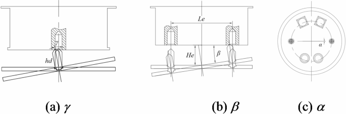
After coarse correction, the maximum radial offset between the active and passive sides is [-Δ1, +Δ1] = [-0.5 mm, + 0.5 mm]. The range of deflection of the passive side around the X-axis is analyzed using the graphical method in positioning analysis coordinate system, as shown in Fig. 12. The limit position occurs when the bottom of the V-groove rotates to the line intersecting the top of the gripping head and the front face. The minimum radius of rotation is r_b=150.32 mm, and after rotating at the maximum angle, the resulting chord length is l_c=2.728 mm. The maximum clockwise rotation angle (negative) around the X-axis is determined as γ = 1.04° using the following formula.

Rotation angle around the X-axis.

According to the graphical method, the maximum counterclockwise (positive) rotation around the X-axis is no more than 1.04°, i.e., the rotation range around the X-axis is [-γ, +γ] = [-1.04°, + 1.04°]. The rotation angle around the Y-axis is [-β, +β] = [-1.04°, + 1.04°] based on the configuration layout. The rotation angle α around the Z-axis depends on the position of the open section of the V-groove relative to the tapered end of the gripping head. The limit occurs when a point on the V-groove’s open section contacts the intersection of the front and rear edges of the gripping head’s tapered end, with the range given as [-α, +α] = [-0.32°, + 0.32°]. Thus, the maximum positional deviation after coarse correction is presented in Table 6.

Precision calibration design

The fine correction function consists of two stages:

(1) Adjustment of the alignment phase, ensuring that the projection of the guide post’s top corner onto the docking surface consistently aligns with the guide holes. One guide hole is designed as a long U-shaped hole, allowing for equivalent analysis of alignment with a circular guide hole, particularly in terms of radial projection deviation. Based on coarse calibration, the radial translation range of the guiding column relative to the guiding hole is [-0.5 mm, + 0.5 mm]. The guiding column and hole are constructed from titanium alloy and aluminum alloy, respectively, with a friction coefficient of approximately 0.3, resulting in a self-locking angle of \(\:\theta\:>\text{arctan}(f)=16.7^\circ\:\)^36,37 The guiding column’s tip angle is restricted to no more than 146.6°, specifically set at 85°. The guide column measures \(\:{\varnothing\:24}_{-0.033}^{0}\) mm, with a tip diameter of approximately 6 mm. The guide hole is Hd=\(\:{{\varnothing}24.2}_{0}^{+0.033}\) mm, with a flare diameter of hd=32 mm, and the center distance between the two semicircles of the long U-shaped holes is 2 mm. The radial offset clearance is \(\:{\rho\:}_{1}=\pm\:\frac{32-6}{2}=13\text{mm}\).

The angular flip is shown in Fig. 13. Rotation around the X-axis will produce Y– and Z-direction deviations of the column head at the tip of the guide column, where the Z-direction deviation will be actively eliminated when the passive end is captured, so only the resulting Y-direction projection translation is considered.

For rotation around the Y-axis, which in the radial direction causes the X-coordinate point of the guide column to converge towards the origin, the offset is equal to the sum of the X-direction offset of the mounting point of the guide column and the X-direction offset produced by the length of the guide column, with a maximum offset:

When rotating around the Z-axis, the guide column translates in the X-axis and Y-axis directions. The offset at the cylindrical head’s tip corresponds to the offset at the guide column’s mounting point center, with a specified maximum offset of:

Therefore the maximum offset in X and Y direction is:

The maximum offset in both the X and Y directions remains within the radial offset tolerance range ρ₁, ensuring that the round head at the tip of the guide column successfully enters the flare of the guide hole.

(2) Precision positioning guide stage: Before the connectors dock, the relative positions of the active and passive sides are adjusted within the required range. The structural design of the guiding column and hole allows for a maximum diameter deviation in the guiding section of \(\:{\rho\:}_{2}=\pm\:\frac{0.2+0.033\times\:2}{2}=\pm\:\text{0.133\,mm}\).

Precision alignment guide illustration.

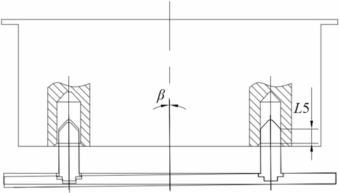
Assuming the guiding section extends to a depth of L5 within the guiding hole, the relative attitude is adjusted within the connector’s tolerance range, as illustrated in Fig. 14. This adjustment ensures that both the maximum displacement deviation, limited to 1.5 mm, and the attitude deviation, limited to 0.9° for β and γ, are maintained below these thresholds. From this configuration, the minimum length of the guiding section can be determined:

The height of the cylindrical cone angle at the tip of the guide column is as follows:

Based on the connector layout design, the protruding docking surface lengths are 26 mm for the floating liquid connector and 24 mm for the floating electrical connector. Therefore, the minimum length of the guide post is:

Assume the guide column length is L7 = 64 mm. Before the connector makes contact, the guiding and positioning length of the guide column, L5, is approximately 24.9 mm. After positioning, the maximum radial deviation between the active and passive sides is [-0.133 mm, + 0.133 mm]. The maximum angular deflection is:

After fine positioning with the double guide columns and before inserting the connector pair, the maximum deviation range between the active and passive sides is detailed in Table 6. This deviation is within the connector’s tolerance requirements. Under the action of the capture jaw drive, the active side continues to approach the passive side, and the final range of positioning accuracy is detailed in Table 6. As shown in the table below, the positioning requirements at each stage are sequentially executed to ensure automatic centering and precise alignment.

Performance analysis of dual-component calibration positioning

During the docking process and mechanical locking of the mechanism, it is crucial to ensure the proper engagement of the floating electrical and fluid connectors between the active and passive sides. This chapter focuses on analyzing and verifying whether the positioning performance indices meet the alignment requirements of the connectors. To achieve this, a generalized structural deviation calculation method is employed, which can analyze and validate deviation ranges for both planar and spatial structures. This method is versatile, allowing the evaluation of coarse calibration deviation ranges as well as fine calibration deviation ranges. The analysis begins with the derivation of a formula for calculating the floating displacement at any point on the positioning structure within the deviation range, based on the principle of two-pin positioning on one side. This planar formula is then extended to three-dimensional space to account for the complexities of spatial structures. The approach ensures that both planar and spatial deviations can be comprehensively assessed. Subsequently, eight typical working conditions are designed, corresponding to the maximum deviations encountered during coarse calibration, as detailed in Table 6. For each condition, the maximum deviations in the three progressive processes—coarse calibration, precision calibration, and final positioning—are analyzed. These deviations are critical for evaluating the docking mechanism’s ability to achieve the necessary alignment and engagement of the floating connectors.

Theoretical analysis of positioning accuracy of double locating pins

As illustrated in Fig. 15(a), the clearance δ between the positioning pin and hole causes the two components to experience random misalignments that are challenging to replicate and correct^38,39,40,41. To analyze the effects of hole-pin float, a coordinate system is set up as shown in Fig. 15b. The locating pin’s coordinate system, XOY(blue), serves as the global coordinate system, while the locating hole’s coordinate system, xoy(red), acts as the local coordinate system.

Double locating pin positioning.

Floating is categorized into main and auxiliary positioning hole pin floating. The floating range of C, at the center of the main positioning hole, forms a circle with a diameter of 2δ. Its floating trajectory is depicted in Fig. 16.

Floating diagram of the primary locating hole.

The positional relationship between the hole center at C and the pin center at O is defined by the coordinates r and θ. The trajectory of C in the XOY is as follows:

Point D, the center of the auxiliary positioning hole, is allowed to float within the Y-axis range λ\(\:\in\:\)(-δ, +δ). This floating motion of D, influenced by the primary positioning hole, involves a composite of translational and rotational movements, as depicted in Fig. 17.

Composite motion of the secondary locating hole center point D.

The trajectory of D, the center of the auxiliary positioning hole, within the XOY is as follows:

In the local coordinate system xoy, the coordinates of any point E(x_E^,, y_E^,) remain constant relative to C, despite the floating of the locating hole pin.

Theoretical analysis of the accuracy of dual-component positioning in six dimensions

The described method extends to the six-dimensional accuracy analysis of the dual-component space. As depicted in Fig. 18, the diagram illustrates the mounting relationship between the active and passive sides. Here, {T} and {C} represent the coordinate systems of the docking surfaces for the active sides a and b, respectively, while {G} and {D} denote the altered coordinate systems.

Illustration of the installation relationship between two components.

If ^GT_T represents the position of {T} relative to {G}, then ^DT_C=(^GT_D)^{−1 G}T_T^TT_C. The center of the passive side’s mounting surface serves as the origin of the world coordinate system, with the distance between the centers of the two docking surfaces being 1642 mm.

Coarse calibration performance analysis

Based on the theory of spatial dual-component positioning accuracy analysis and the results of the maximum position deviation from single-component coarse correction, the position deviation of the active side b relative to the passive side can be seen in Table 7.

The Z-direction displacement deviation of component b, caused by the Y-axis deflection of the winding member a, reaches up to 29.8 mm. Similarly, the Y-direction displacement deviation due to the Z-axis deflection reaches up to 9.17 mm. These deviations should be further constrained by the coarse correction of the capturing jaws of component b. Therefore, subsequent actions involving both components should only proceed after the coarse correction of the capturing jaws for both component a and component b is completed. The maximum positional deviation when the dual components are coarsely corrected together is displayed in Table 8.

Fine positioning performance analysis

Like the coarse positioning analysis, the maximum positional deviation of component b is determined based on the finely corrected maximum deviation of component a. This deviation is detailed in Table 9.

The maximum Z-direction displacement deviation of component b, caused by the Y-axis deflection of winding member a, is up to 1.72 mm, similarly for the Y-direction due to the Z-axis deflection. The coarse correction by component b’s capture jaws limits the Y-direction deviation to less than 0.5 mm, and the Z-direction deviation decreases gradually as the capture jaws close. Consequently, there is no need for a guide column to position component b. The maximum positional deviation of the dual-components after fine positioning is displayed in Table 10.