Wind induced structural response analysis of photovoltaic tracking supports by unidirectional fluid structure coupling

The motion of a continuous fluid medium is governed by the principles of classical mechanics and fluid dynamics. Considering the actual operating conditions of the photovoltaic tracking support structure, the fluid is assumed to be continuous, homogeneous, and incompressible, while the effects of temperature and the energy equation are neglected. Under a fixed coordinate system, the governing equations of fluid motion²² are expressed as follows:

where, \(\rho\) is the fluid density, in kg/m³; \(t\) is the time, in seconds; \(v\) is the velocity vector, in m/s; \(\nabla\) is the divergence operator, representing the divergence of a vector field; \(\tau\) is the stress tensor, in Pa; \(f_{B}\) is the body force vector, in N/m³.

The solid finite element governing equation is:

where, \(\rho_{s}\) is the solid density, in kg/m³; \(\mathop d\limits^{..}_{s}\) is the acceleration vector of the solid, in m/s²; \(\nabla\) is the divergence operator, which represents the divergence of a vector field; \(\sigma_{s}\) is the Cauchy stress tensor, in Pa; \(f_{s}\) is the body force vector, in N/m³.

At the fluid–solid interface, the continuity conditions for stress, displacement, and other relevant variables must be satisfied, ensuring the equality or conservation of these quantities. This requirement is expressed by the following equations:

where, \(\tau\) is the stress at the interface, in Pa; \(n\) is the directional cosine at the interface subscript; the subscript \(f\) denotes the fluid; the subscript \(s\) denotes the solid; \(d\) is the displacement at the interface, in m.

Development of the Fluid–Structure Interaction model and flow field configuration

This study is based on a multi-row photovoltaic (PV) tracking support system installed at a solar power station in Hefei, Anhui Province. A simplified numerical model of the PV support structure was developed for simulation purposes by omitting detailed components such as bolts, threads, and screw holes. The model adopts a 5-row × 5-column array configuration, representing a typical setup that achieves optimal power generation efficiency when the PV panels are directly aligned with the sun. The PV tracking system is capable of automatically adjusting the panel tilt angle in response to the sun’s incident angle.

To better reflect practical engineering scenarios, three representative tilt angles 15°, 30°, and 45° were selected for analysis. These angles correspond to typical operational conditions, representing low, moderate, and near-maximum tilt configurations widely used in current PV installations. Among them, 30° is the commonly adopted optimal installation angle at the study site, while 15° and 45° represent the operational extremes in real-world tracking systems, associated respectively with the minimum tilt state and the most wind-sensitive condition.

Accordingly, this study focuses on analyzing the wind pressure distribution and wind-induced response characteristics at these three tilt angles, providing valuable engineering insights and practical relevance. The analysis includes the pressure distribution under the most unfavorable along-wind condition (0° wind direction) and the most unfavorable reverse-wind condition (180° wind direction). In-depth investigation is further conducted under the typical working condition of 30° tilt angle with 0° wind direction. The array configuration of the PV tracking support system is illustrated in Fig. 2.

Schematic of the photovoltaic array layout.

The structural components of the photovoltaic tracking support system studied in this paper include photovoltaic panels and supporting elements. Photovoltaic modules are made of composite materials, such as Glass Fiber Reinforced Polymer (GFRP) or Carbon Fiber Reinforced Polymer (CFRP). These materials offer high strength, low weight, and excellent corrosion and weather resistance, allowing them to withstand wind loads effectively and provide long-term stability. The purlins and main beams are constructed from S350GD steel, which offers high strength and excellent corrosion resistance, making it well-suited for lightweight structural applications. In contrast, the columns require greater load-bearing capacity and stability; therefore, Q355B structural steel, known for its enhanced toughness and higher tensile strength, is selected to ensure overall structural safety and reliability. The components of the photovoltaic array are interconnected as follows: photovoltaic panels are bolted to the purlins, which are similarly bolted to the posts. Each row of photovoltaic panels is closely arranged within the support structure, with the panels secured by supporting frames and connecting bars to ensure stability under wind loads. These connections ensure the overall structural stability of the photovoltaic support system and effectively transfer wind loads and other external forces.

Figure 3 illustrates the arrangement and dimensions of the photovoltaic panels and their supporting components. To simplify the observation of the supporting components’ installation method, the photovoltaic panels on both sides are omitted for clarity. In the figure, ① denotes the purlin; ② denotes the main beam; ③ denotes the photovoltaic panel; ④ denotes the post, which supports the entire structure and is connected to the ground. The dimensions in the figure are as follows: (a) purlin cross-sectional dimensions; (b) main beam cross-sectional dimensions; (c) post cross-sectional dimensions; (d) photovoltaic panel cross-sectional dimensions.

Schematic diagram of the structure and dimensions of the photovoltaic module (unit: mm).

The photovoltaic support structure is analyzed using a fluid–structure coupling method for transient analysis. Shell elements are employed to model the photovoltaic panels, while solid elements model the support components (purlins, main beams, posts) to accurately simulate the structural response of the components under wind load. To model the structural damping effect, the Rayleigh damping model is used, which dissipates energy by adjusting the proportional factors of the mass and stiffness matrices. This ensures stable and accurate analysis results, particularly under the influence of pulsating wind loads.

To ensure adequate flow field development and simulation accuracy, the blockage ratio in this study is set to 2.5%, which is below the standard 3% threshold commonly recommended in the literature²³. This configuration is based on widely adopted practices in previous studies and effectively minimizes the interference caused by blockage effects on flow field distribution. Moreover, since the blockage ratio primarily affects the overall wind speed distribution and has limited influence on the local wind load characteristics of the panels, this setting does not compromise the robustness of the simulation results and conclusions. The computational domain is divided into two parts: the outer flow field and the refined subdomain (local refinement zone). The dimensions of the entire fluid domain and the corresponding mesh division are shown in Fig. 4 and Fig. 5, respectively.

Schematic of the fluid domain dimensions.

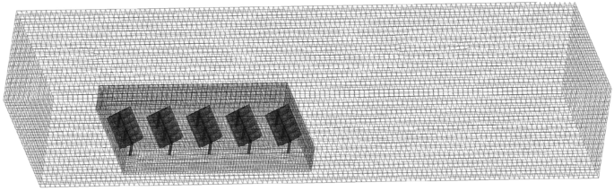
Fluid domain grid division.

In this study, a hexahedral mesh is used for the meshing of the entire flow field. Hexahedral meshes significantly enhance computational accuracy, efficiency, and numerical stability. Mesh density is a key factor influencing the accuracy of simulation results. In this study, five different mesh schemes were evaluated, and mesh independence analysis was conducted based on the average turbulent kinetic energy on the windward surface of the central photovoltaic module in the array, selected as a representative aerodynamic parameter. Turbulent kinetic energy effectively reflects the intensity and instability of the local flow field and serves as a sensitive and representative indicator for identifying wind load-prone regions. Although pressure coefficients and structural responses are also important, preliminary verification indicated that variations in pressure distribution and structural loading in critical areas were minimal across different mesh schemes. Therefore, to ensure simulation accuracy while improving computational efficiency, turbulent kinetic energy was adopted as the primary metric for the mesh independence assessment, as shown in Fig. 6.

Grid independence verification.

In this study, although the RANS turbulence model typically requires fewer grid elements (typically in the range of millions), extremely fine grids are employed in the boundary layer region around the photovoltaic panels to precisely capture the complex wind flow features around the photovoltaic support. These refined grids enable more accurate simulations of the variation in wind load distribution and the local fluid characteristics, ensuring that the simulation results accurately represent the actual conditions.

At 11.34 million mesh elements, the average turbulent kinetic energy exhibits negligible variation and stabilizes as the mesh resolution increases. The deviation from the results at 14.56 million elements is merely 1%, indicating that further mesh refinement has an insignificant impact on the results. To ensure the reliability of the computational results while conserving computational resources, the final model with 11.34 million elements and 10.95 million nodes was adopted.

In this simulation, the entire model was developed on the ANSYS platform. The wind field in the fluid domain was simulated using Fluent, while the structural domain was analyzed in ANSYS Mechanical to evaluate the dynamic response of the photovoltaic support structure. A one-way fluid–structure interaction (FSI) approach was employed, in which wind pressure loads obtained from the fluid analysis were transferred as boundary conditions to the structural domain for response analysis. The structural deformation and displacement did not exert any feedback on the fluid domain.

Boundary conditions and computational methods

Inlet Boundary Conditions: The inlet is specified as a velocity inlet. An integral fitting function and an exponential function are employed to develop a stochastic wind time-series control algorithm for the wind field inlet. The wind velocity boundary layer is implemented using Fluent/UDF.

where, \(v_{x}\) is the inlet velocity, in m/s; \(v_{0}\) is the 50-year basic wind speed at the model location, in m/s; \(v_{j}\) is the pulsating wind speed, in m/s.

According to the Code for Loads of Building Structures²⁴, the basic wind pressure for the photovoltaic support structure is determined based on the 50-year return period wind pressure in the study area. As indicated in Table E.5 of the Code for Loads of Building Structures, the 50-year return period wind pressure in Hefei is 350 Pa. The relationship between wind speed and dynamic pressure is given by the following equation:

where, \(\omega_{0}\) is the 50-year recurrence basic wind pressure in Hefei, taken as 350 Pa; \(\rho\) is the air density, taken to be 1.25 kg/m³; \(v_{0}\) is the 50-year basic wind speed in Hefei, calculated to be 23.25 m/s, and for safety, the value is taken as 25 m/s.

In this study, the inflow wind speed is assumed to be uniform, with a wind speed of 25 m/s at a reference height of 10 m. Although the actual wind speed distribution adheres to the wind profile of the atmospheric boundary layer, typically represented by logarithmic or exponential distributions, where wind speed varies with height and is influenced by surface roughness and other factors, the assumption of a uniform wind speed distribution is made to simplify the model and focus on wind-induced response analysis. This assumption implies constant wind speed across the entire computational domain, thereby avoiding the complexity of calculating wind profiles.

Additionally, the inlet boundary conditions must capture the turbulent characteristics of the incoming wind. The calculation formula is as follows:

where, \(K\) is the turbulent kinetic energy, in m²/s²; \(u^{\prime }\), \(v^{\prime }\), and \(\omega^{\prime }\) are the turbulent velocity fluctuation components in the x, y, and z directions, respectively. These components are obtained by solving the velocity fluctuation equations of the turbulence model. Specifically, the calculation of, \(u^{\prime }\),\(v^{\prime }\) and \(\omega^{\prime }\) relies on the correlation of the time-averaged velocity and fluctuating velocity fields in the turbulence model, and is derived through solving the turbulence energy and dissipation equations; \(\varepsilon\) is the turbulent dissipation rate, in m²/s³; \(C_{u}\) is the empirical constant, taken as 0.09; \(l\) is the turbulent length scale, in meters.

A standard atmospheric pressure outlet is applied at the outlet. This setting effectively simulates the pressure balance between the surface of the photovoltaic module and the atmosphere, preventing unrealistic pressure gradients at the outlet, thereby enhancing the accuracy of the simulation results. Symmetric boundary conditions are applied to the top and lateral walls to simplify the model and reduce computational effort, ensuring that no unwanted wall effects influence the simulation process. The flow surface of the photovoltaic module and the bottom, representing the ground, are assigned no-slip boundary conditions to realistically model the interaction between the fluid and the surface, ensuring that the fluid velocity at the boundary is zero, as required by the actual physical conditions.

In this study, the turbulence model chosen is the standard k-epsilon model, which is capable of simulating boundary layer flow and turbulence characteristics with high accuracy, while offering relatively high computational efficiency. This model has been widely used in similar wind flow simulations and has proven effective at accurately capturing the interaction between the airflow and the photovoltaic structure²⁵.

The convergence tolerance is set to 10⁻⁴, ensuring both sufficient accuracy and computational efficiency. The time step is set to 0.01 s, with 20 iterations per step. This configuration has been validated through preliminary tests to ensure numerical stability and accuracy. The simulation duration is 40 s, which is adequate to capture the impact of wind load on the photovoltaic modules and provide stable dynamic response data.